
The following course material was transcribed from copies found in Franco Modigliani’s papers at the Economists’ Papers Archive in the David M. Rubenstein Rare Book & Manuscript Library of Duke University. These items are also available in a scanned .pdf file at the Cowles Foundation website at Yale. Modigliani’s original mimeographed copy is for the most part much more legible than the on-line scanned copy at the Cowles Foundation. This is particularly true for the “terminal examination” questions. Over forty pages of typescript for the lectures are also found in the original Cowles Commission Discussion paper.
More on Jacob Marschak can be found in Robert W. Dimand’s “Keynesian Economics at the Cowles Commission” (Review of Keynesian Studies, vol. 2, 2020, pp. 22-25).
________________________
J. Marschak. INTRODUCTION TO ECONOMETRICS
Economics 314
Spring 1949.
314. Introduction to Econometrics: Statistical testing of economic theories. Numerical estimation of demand and cost functions and other functions occurring in the theory of the firm and household, the theory of markets and the theory of national income. Estimation of economic models. Statistical prediction under conditions of changing economic structure and policy. Prerequisites: Econ 310, 311, 312 or equiv. Win [sic] TuTh 3-4:30; Marschak.
Source: University of Chicago.The College and the Divisions, Sessions of 1948-1949. In Announcements Vol. XLVIII (May 25, 1948) No. 4, p. 250.
________________________
INTRODUCTION TO ECONOMETRICS
20 Lectures given at the University of Chicago in Spring, 1949*
Cowles Commission Discussion Papers, Economics: 266
[*To be used jointly with 24 Lectures (same title) given at the University of Buffalo in Spring, 1948.]
Part I. Non-stochastic economics [11 lectures]
- Best policy. Goal variable; non-controlled, controlled, strategic variables.
- Exogenous variables and structural parameters. Types of prediction.
- Determining the structure from theory and data.
- An example.
- Econometric “pitfalls” due to disregarded variables or relations. Non-idenifiable structures.
- [continued]
- The identification, continued
- Why does the identification problem arise in non-experimental sciences?
- Discussion of earlier problems.
- Discussion of earlier problems. [continued]
- When need we know the structure?
Part II. Stochastic economics: Population properties [8 lectures]
- Joint distributions, non-parametric.
- Mid-term examination.
- Parameters of joint distributions.
- Least-squares property of coefficients of linear regression. Properties of normal distributions.
- Exogenous and endogenous variables in stochastic economics.
- Identification and determination of structure by the method of reduced form: examples.
- More examples.
- Motion of an economic variable. Dynamic models. The assumption of independent successive disturbances and its implication.
Part III. Stochastic economics: Sample properties [1 lecture]
- Useful properties of certain least squares and maximum likelihood estimators. Obtaining maximum likelihood estimates of structure from those of reduced form.
Recommended reading.
Attached Materials**
J. Marschak, “Economic Structure, Path, Policy and Prediction”
__________, “Statistical Inference from Non-Experimental Observations—an Economic Example”
G. Hildreth, “Problems in the Estimation of Agricultural Production Functions”
[**As far as available.]
* * *
READING MATERIAL TO BE USED IN COURSE ON INTRODUCTION TO ECONOMETRICS,
SPRING QUARTER, 1949
- Allen, R. G. D., Mathematical Analysis for Economists.
- American Economic Association, “Survey of Contemporary Economics” (Blakiston Co., 1949).
- Haavelmo, T., “The Probability Approach to Econometrics” (Supplement to Econometrica, 194) .
- Haavelmo, T., “Quantitative Research in Agricultural Economics,” Journal of Farm Economics, Vol. 29, No. 4, November, 1947.
- Girshick, M. A., and T. Haavelmo, “Statistical Analysis of the Demand for Food,” Econometrica, Vol. 15, No. 2. April, 1947.
- Klein, Lawrence R., “The Use of Econometric Models,” Econometrica, April, 1947.
- Haavelmo, T., “Methods of Measuring the Marginal Propensity to Consume,” Journal of the American Statistical Association, March, 1947.
- Klein, Lawrence R., “A Post-Mortem on Transition Predictions,” Journal of Political Economy, August, 1946.
- Marschak, J., L. Hurwicz, Abstracts of papers: Econometrica, April, 1946, pp. 165-170.
- Koopmans, T., “Statistical Estimation of Simultaneous Economic Relations,” Journal of the American Statistical Association, Vol. 40, December, 1945.
- Marschak, J. and William H. Andrews, “Random Simultaneous Equations and the Theory of Production,” Econometrica, Vol. 12, No. 3-4, July-October, 1944.
- Marschak, J., “Money Illusion and the Demand Analysis,” The Review of Economic Statistics, 25, February, 1943.
- Marschak, J., “Economic Structure, Path, Policy, and Prediction,” American Economic Review, Vol. 37, May, 1947, pp. 81-84. Lil.
- Marschak, J., “Statistical Inference from Non-Experimental Observations,” Econometrica, January, 1948, p. 53.
- Hurwicz, L., “Some Problems Arising in Estimating Economic Relationships,” Econometrica, Vol. 15, July, 1947.
- Tinbergen, J., “Business Cycles in the U.S.A. 1919-1932” (Statistical Testing of Business-cycle Theories. II), League of Nations, Geneva, 1939.
- Koopmans, T., “Measurement without. Theory,” Review of Economic Statistics, 29, August, 1947.
* * *
J. Marschak.
INTRODUCTION TO ECONOMETRICS
Economics 314, Spring 1949.
Terminal Examination
Note: Try to answer all 4 problems first, omitting the questions (III) in problems 1 and 4. Answer the questions (III) if time remains.
Problem 1. The quantity x and the price p of a perishable farm product (each measured from its population mean) are determined as in the following model (subscripts indicate time):
(1.1) Demand: xt = αpt + ut
(1.2) Supply: xt = βpt-1 + ut
(1.3) The disturbance ut is not autocorrelated; nor is vt.
Show
(I) How to estimate α for a long time series.
(II) What other structural parameters are present?
(III) (If time remains): How would you estimate those other parameters?
Problem 2. The model of the previous problem is modified as follows:
(2.1) Demand: xt = αpt + ut (ut not autocorrelated)
(2.2) Price fixation: 
Show
(I) How to estimate α and σuu?
(II) Is the estimate of α the same as in the previous problem?
Problem 3. National income y, consumption c, and annual (saving) investment i are all measured in dollars of constant purchasing power, and
(3.1) c = αy + β + u ;
(3.2) E(u);
(3.3) i = y – c (an identity);
(3.4) i is exogenous.
(I) Show how to estimate α, β, σuu from a long time series of data on y, c, i.
(II) Suppose y, c, i denote the income, consumption and saving of an individual family which can control its savings but not its income. How does this modification affect the model and the estimation procedure from a time series of family data, or from a survey of a large number of families?
Problem 4. A survey of very large number T of firms belonging to the same industry but located in places with different wage-rates w1, …, wT has been made. The price p of the product is the same for all firms. Wage-rates and price are fixed independently of the firms’ action. The output Xt of each firm depends on labor used only, Nt, according to the formula
(4.1) 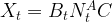
(the elasticity A being the same for all firms.) Hence,
(4.2) xt = bt + Ant, t = 1, …, T
where the small letters (except for t) stand for the logarithms. Further assume that each firm pushes its output to the point where, apart from a random deviation, the ratio 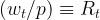
(4.3) Rt = (dXt/dN)⋅Ct, t = 1, …, T
where Ct is a random percentage deviation. Hence
(4.4) Rt = 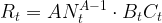
(4.5) rt = a + bt + ct + (A-1)nt, t = 1, …, T,
where again small letters indicate logarithms.
Questions:
(I) How to estimate A?
(II) What other structural parameters are present?
(III) (If time remains): How to estimate those?
Source: Duke University. David M. Rubenstein Rare Book & Manuscript Library. Economists’ Papers Archive. Franco Modigliani Papers, Box T1, Folder “Jacob Marschak’s Courses, 1940-1949.”
Image Source: Carl F. Christ. History of the Cowles Commission, 1932-1952