
We turn our attention now to relatively recent Macroeconomic Theory. The immediately preceding post provides a transcription of the Spring 1991 General Examination in Microeconomic Theory at Harvard.
This post represents the second artifact from the Abigail Wozniak collection of Harvard graduate economics general examinations from Spring 1991 through Spring 1999. Future installments will be posted, though not on a regular schedule.
From the different formatting and fonts seen in the original copies, we can conclude that Part I (questions 1-3), Part II (questions 4-6), Part III (questions 7-9) were each written by different sets of examiner(s).
___________________________
HARVARD UNIVERSITY
DEPARTMENT OF ECONOMICS
ECONOMICS 2010d: FINAL EXAMINATION and
GENERAL EXAMINATION IN MACROECONOMIC THEORY
SPRING, 1991
Instructions for all Economics Department graduate students:
The examination will last four hours.
Answer all three parts of the examination (Parts I, II and III).
Within each part, answer any two of the three questions given (so that, in all, you will answer six questions).
Use a separate bluebook for each question. Clearly indicate the question number and your identification number on the front of each bluebook.
Do not indicate your name on any bluebook you submit.
Instructions for all other students:
The examination will last three hours.
Answer Parts II and III only. Within each part, answer any two of the three questions given (so that, in all, you will answer four questions).
Use a separate bluebook for each question. Clearly indicate the question number and your name on the front of each bluebook.
PART I
Question 1
“Old Keynesian” models were often criticized by their detractors for their apparent reliance on counter-cyclical real wages to generate fluctuations in output. Write a well crafted essay giving several examples of how more modern models (both Keynesian and non-Keynesian) have dealt with this issue. Explain the mechanism by which each model yields output fluctuations without counter-cyclical real wage fluctuations.
Question 2
Suppose that the simplest Lucas model describes the economy:
(1) 
(2) 
where t-1pt represents the mathematical expectation as of period t-1 of the price in period t, and 

Suppose, however, that private agents, in their ignorance, believe that the economy is described by (1) and:
(3) 
where 
(a) Will this ignorance lead to any real effects of anticipated money under any of the following monetary policies? “Where relevant, assume the central bank knows that (2) is true but that people believe (3).)
(4.1) 
(4.2) 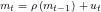
(4.3) 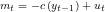
Here ut is a random error, and 
(b) Now suppose agents make a different mistake. They think the supply function is
(5)

That is, they know the parameter, but get the lag structure wrong. Answer the same question again.
(c) Give a brief intuitive explanation of why you obtain different answers in parts (a) and (b).
Question 3
Consider the following simple growth model:
The economy is comprised of a single representative agent, who divides his labor between two activities. A fraction 

Suppose that the production function for consumer goods is.

where kt denotes the capital stock as of time t.
The evolution of the capital stock is given by,

where 

(a) If 

(b) Suppose that consumer preferences are given by,

Where 

Before calculating this algebraically, explain the basic trade-offs involved in selecting and optimal 

(c) How does an increase in the depreciation rate 
PART II
Answer any two of the following three questions. Be sure to use a separate bluebook for each answer.
- Suppose that a nation’s government seeks to influence its level of aggregate demand so as to keep it as close as possible to the “full employment” level of output, which is determined independently of government actions. Suppose also that the government has two ways of affecting aggregate demand. Government spending closely and reliably influences aggregate demand; money growth also influences aggregate demand, but in a highly unpredictable manner. At the same time, there is a specific level of government spending that is deemed appropriate for reasons having nothing to do with its effect on aggregate demand; by contrast, the rate of money growth is of no consequence except insofar as it causes aggregate demand to be above or below “full employment” output. How can the government take account of these considerations in its conduct of fiscal and monetary policy?
- What aspects of economic behavior determine whether monetary policy should tighten, ease, or remain unchanged when the economy experiences an adverse shock affecting its aggregate ability to supply goods and services on the basis of given labor and capital inputs? Be specific about the policy objective that your answer assumes.
- Under what circumstances will a tax-and-transfer system intended to buffer the economy against shocks (of whatever origin) be unable to affect the distribution describing real economic outcomes? Show clearly that the set of assumptions you posit is sufficient for this “ineffectiveness” result. What are the major correspondences and contrasts between this set of assumptions and the conditions under which actual tax-and-transfer systems typically function in most industrialized economies? What conclusions do you draw from any contrasts?
Part III
Question 7
Consider the following model of a small open economy under flexible exchange rates:
I = I0 – r,
S = r,
X = R,
M = –R,
F = –
[S– (G– T)] – I = X – M,
F = X – M,
Where I = domestic investment, S = domestic private saving, X = exports, M = imports, F = capital outflow, G = government spending, T = tax revenues, r = domestic real interest rate, and R = real exchange rate. I0 is a shift variable representing investment demand shocks, and 

- Suppose that fiscal policy is exogenous, in the sense that
G – T = G0 – T0, G0, T0 given.
What are the equilibrium effects of an investment shock (a change in I0) on national saving and investment? Is a positive investment-national saving relation an indicator of a lack of perfect capital mobility? Explain.
- Suppose now that fiscal policy is endogenous, in the sense that
G – T = [G0 + 
where 0 <
- Can the presence or lack of a crowding out effect of fiscal policy (resulting from changes in G0) be used to empirically discriminate between the exogeneous and endogenous policy hypotheses? Why or why not?
- Comment on the potential theoretical and empirical implications of this exercise.
Question 8
The “twin deficits” hypothesis asserts that U.S. Federal budget deficits are responsible for U.S. trade deficits.
- Present two models, one which supports and one which invalidates, this hypothesis.
- How could a proponent of the model which does not support the twin deficit hypothesis account for the recent coincidence of budget and trade deficits?
- How would you test empirically each of your proposed models?
Question 9
What are the effects on consumption and capital accumulation of i) a proportional labor income tax, and ii) a proportional capital income tax in:
- A life-cycle (overlapping generations) model;
- An economy with infinitely-lived consumers.
Source: Department of Economics, Harvard University. Past General Exams, Spring 1991-Spring 1999, pp. 89-94. Private copy of Abigail Waggoner Wozniak.
Image Source: View of Widener Library from Harvard Campus, Cambridge, Mass. from Boston Public Library, Tichnor Brothers Collection of Massachusetts Postcards.